“The cleanest kWh is a kWh not used” has been the energy efficiency (EE) battle cry for decades. And utilities are delivering on that in myriad ways: innovating new program designs while continuing to improve EE savings nationwide. But we see a big opportunity to deepen energy savings nationwide still untapped: improved EE program targeting based on individual home savings potential.
Today, most, but not all, EE programs target all homes equally, due to legacy effects in the way programs are structured. In some programs, psychographic or demographic targeting is used to fine tune messaging and outreach, but that is primarily a marketing exercise. This approach made sense in a world where you couldn’t estimate the savings you’d get until after the treatment. Now, with the ability to prioritize high potential-savings homes, that paradigm has shifted. It’s time you take advantage of these new capabilities, for the benefit of all ratepayers.
Let’s look at how much value your utility could realize by analyzing a hypothetical EE program with help from Bidgely’s Insights Engine, our AI-powered tool enabling utilities to find the highest potential homes for any DSM program.
Why EE Programs Struggle With Efficiency
For this example, we will look at an A/C retrofit program, with some simplifying assumptions*. Customers are provided a flat $800 rebate to replace central A/C units in single family homes with SEER 16 rated units.
The program replaces 3,000 units a year, costing the ratepayers $3.2M ($2.4M in rebates and $0.8M in admin and marketing).
The savings calculation is based on the current industry standard—a simplified deemed savings formula—for central A/C retrofits:
![]()
Where:
- Full Load Hours (FLH) is the number of hours per year of operation, in this case we used 1,400
- Capacity is the cooling capacity of the unit in BTU/hr
- SEER is the Season Energy Efficiency Rating of the existing unit and efficient replacement unit, respectively
Focusing just on one-year savings, this histogram shows the distribution in savings potential from home to home based on an analysis of 1,000 randomly chosen single family homes.

Take a look at savings potential per user, and more importantly, what that means financially for the program.

The cost to serve each participating home is the same $800 rebate, but the actual savings generated differ significantly from home to home. So the more a program does to shift participation from lower-saving homes to higher-saving homes, the more cost-effective the program will be. Let’s play out a few different scenarios to illustrate this, using our Insights Engine just as a program implementer would to design the most effective program.
How to Save More On Your Next EE Program
We start with a baseline scenario, a random sampling of homes.
The real-world scenario is probably closest to how your EE programs look now: people somewhat self-select into the most relevant programs for them. We make a proxy of this by saying that the bottom quartile of savers only makes up 10% of participants, and the fourth quartile of savers makes up 40% of participants. The rest of the participants are randomly chosen.
In the targeted scenario, the utility is able to direct the program aggressively to the top quartile savers, and they will make up ~60% of participants, with the remaining 40% randomly drawn from the rest of the homes. This represents a situation where the utility successfully moves the needle towards higher savers, but can’t exclude other participants, so many lower saving homes will still participate to some degree.
In each scenario, 3,000 homes are treated per year, with the same $3.2M annual budget.
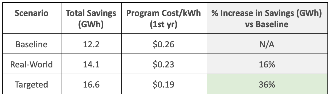
As you can see, the targeted scenario generates about 36% more savings than the baseline scenario and 18% more savings than the real-world scenario, with the same budget: a substantial step-change in overall program performance.
This analysis applies to every EE and DR program. The magnitude of value created will differ by program type and geography, but what holds is that participants’ savings are always going to vary, and there will always be a long tail of very high potential-savings homes that should be courted at almost any cost.
Targeting in the Real World
We perceive two major objections to this approach from the market. First, the program often has to be open to every ratepayer, making it hard to only target homes with the highest savings potential. And second, higher consumption homes tend to be wealthier, so this approach results in funneling rebates towards already wealthy homeowners.
But, both of these problems can be solved through explicit program design. Having more cost-effective programs gives you the flexibility to accommodate other goals while still achieving a positive total resource cost (TRC). For example, programs might use those savings to expand low- to middle-income offerings. In the above scenario, this might play out by only having to serve 2,500 high savings homes to hit the GWh goals (instead of the original 3,000), then using the rest of the rebates to treat 500 disadvantaged customers.
Rather than accepting worse program performance to accommodate implicit program goals, such as serving a wide array of customer types, make those other goals explicit and work them into your program design, or create price signals like performance incentives that reward participants who help you hit your program goals. With a potential ~20% increase in savings at stake for the same budget, you’ve got a lot of room to accommodate other goals.
*Methodology
We analyzed 1,000 randomly and anonymously selected single family homes from EIA’s Hot/Dry region. Using energy disaggregation based on smart meter consumption data coupled with home size, we estimated:
- Total kWH used for A/C (disaggregation algorithm)
- Power draw for unit in KW (disaggregation algorithm)
- Cooling capacity of unit (assumes 1 ton cooling per 600 sqft, or 20 BTU/hr/sqft)
- SEER rating of the existing unit (calculated with power draw & cooling capacity)
For simplifying assumptions, we assumed that multiple A/C units for one home would roll up into one unit—if a home upgrades one A/C, they upgrade them all. This won’t necessarily be true in the real world, but on average it calculates to the same outcome.
We also assumed that the cooling capacity of the unit will be the same after retrofit, and did not factor in actual consumption changes due to weather or deterioration effects.
To determine deemed savings potential for each home, we used our estimate for cooling capacity of the A/C unit, multiplied by the difference of the inverse SEER rating (1/existing SEER – 1/upgraded SEER) to get the difference in power draw in kW for each unit. We then multiplied this by the deemed savings Full Load Hours running to estimate (1,400).
Learn More about Bidgely’s Insights Engine
0 Comments